Transformed Data

VegaFusion supports extracting the transformed data for an Altair Chart using the vegafusion.transformed_data() function. This is particularly useful when building a chart that includes a pipeline of transforms, as it’s now possible to see the intermediate results of each transform.

Example: Top K

Here is an example, based on the Top-K plot with Others example from the Altair documentation, of how transformed_data() can be helpful when building a complex chart.

First, create an Altair Chart wrapping the data source URL.

import altair as alt
import vegafusion as vf

source = "https://cdn.jsdelivr.net/npm/vega-datasets@v1.29.0/data/movies.json"
chart = alt.Chart(source)

The transformed_data() function can be used on this empty chart to access a preview of the data that is available at the URL. Here the row_limit argument is used to limit the result to 3 rows and the DataFrame is transposed to make it easier to read.

vf.transformed_data(chart, row_limit=3).T

	0	1	2
Title	The Land Girls	First Love, Last Rites	I Married a Strange Person
US_Gross	146083	10876	203134
Worldwide_Gross	146083	10876	203134
Production_Budget	8000000	300000	250000
Release_Date	Jun 12 1998	Aug 07 1998	Aug 28 1998
MPAA_Rating	R	R
Distributor	Gramercy	Strand	Lionsgate
IMDB_Rating	6.1	6.9	6.8
IMDB_Votes	1071.0	207.0	865.0
Major_Genre		Drama	Comedy
Rotten_Tomatoes_Rating	nan	nan	nan
Source
Creative_Type
Director
US_DVD_Sales	nan	nan	nan
Running_Time_min	nan	nan	nan

The first step of making this chart is to compute the average worldwide gross of all the movies for each director. This can be accomplished with the Altair Aggregate Transform.

chart = (
    alt.Chart(source)
    .transform_aggregate(
        aggregate_gross='mean(Worldwide_Gross)',
        groupby=["Director"],
    )
)
vf.transformed_data(chart, row_limit=5)

	Director	aggregate_gross
0		3.59284e+07
1	Christopher Nolan	3.44251e+08
2	Roman Polanski	5.13407e+07
3	Richard Fleischer	2.27635e+07
4	Blake Edwards	5e+06

Next, the directors are ranked by average gross in descending order. This can be accomplished with the Altair Window Transform

chart = (
    alt.Chart(source)
    .transform_aggregate(
        aggregate_gross='mean(Worldwide_Gross)',
        groupby=["Director"],
    ).transform_window(
        rank='row_number()',
        sort=[alt.SortField("aggregate_gross", order="descending")],
    )
)
vf.transformed_data(chart, row_limit=5)

	Director	aggregate_gross	rank
0	David Yates	9.37984e+08	1
1	James Cameron	8.29781e+08	2
2	Carlos Saldanha	7.69293e+08	3
3	Pete Docter	7.31305e+08	4
4	Andrew Stanton	7.00319e+08	5

Then, a new column is added that contains the director’s name for the top 9 ranked directors and “All Others” for the remaining directors. This can be accomplished using the Altair Calculate Transform.

chart = (
    alt.Chart(source)
    .transform_aggregate(
        aggregate_gross='mean(Worldwide_Gross)',
        groupby=["Director"],
    ).transform_window(
        rank='row_number()',
        sort=[alt.SortField("aggregate_gross", order="descending")],
    ).transform_calculate(
        ranked_director="datum.rank < 10 ? datum.Director : 'All Others'"
    )
)
vf.transformed_data(chart, row_limit=12)

	Director	aggregate_gross	rank	ranked_director
0	David Yates	9.37984e+08	1	David Yates
1	James Cameron	8.29781e+08	2	James Cameron
2	Carlos Saldanha	7.69293e+08	3	Carlos Saldanha
3	Pete Docter	7.31305e+08	4	Pete Docter
4	Andrew Stanton	7.00319e+08	5	Andrew Stanton
5	David Slade	6.88155e+08	6	David Slade
6	George Lucas	6.73577e+08	7	George Lucas
7	Andrew Adamson	6.43134e+08	8	Andrew Adamson
8	Peter Jackson	5.95566e+08	9	Peter Jackson
9	Richard Marquand	5.727e+08	10	All Others
10	Eric Darnell	5.66099e+08	11	All Others
11	Roland Emmerich	4.5506e+08	12	All Others

Finally, this dataset is ready to be encoded as a bar mark:

import altair as alt
import vegafusion as vf

vf.enable()

source = "https://cdn.jsdelivr.net/npm/vega-datasets@v1.29.0/data/movies.json"
chart = (
    alt.Chart(source)
    .transform_aggregate(
        aggregate_gross='mean(Worldwide_Gross)',
        groupby=["Director"],
    ).transform_window(
        rank='row_number()',
        sort=[alt.SortField("aggregate_gross", order="descending")],
    ).transform_calculate(
        ranked_director="datum.rank < 10 ? datum.Director : 'All Others'"
    ).mark_bar().encode(
        x=alt.X("aggregate_gross:Q", aggregate="mean", title=None),
        y=alt.Y(
            "ranked_director:N",
            sort=alt.Sort(op="mean", field="aggregate_gross", order="descending"),
            title=None,
        ),
    )
)
chart

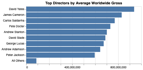
The exact value of each bar can be accessed by applying transformed_data() to the final chart (which includes the implicit transforms in the bar mark encoding).

vf.transformed_data(chart)

	ranked_director	mean_aggregate_gross
0	David Yates	9.37984e+08
1	James Cameron	8.29781e+08
2	Carlos Saldanha	7.69293e+08
3	Pete Docter	7.31305e+08
4	Andrew Stanton	7.00319e+08
5	David Slade	6.88155e+08
6	George Lucas	6.73577e+08
7	Andrew Adamson	6.43134e+08
8	Peter Jackson	5.95566e+08
9	All Others	8.87602e+07

Datetime Timezone

Datetime columns will be returned in the local timezone returned by the vegafusion.get_local_tz() function. If not overridden using vegafusion.set_local_tz(), this will be the local timezone of the Python kernel.

For example:

import vegafusion as vf
import altair as alt
from vega_datasets import data

# Manually set timezone to Seattle's since this a seattle weather
# dataset
vf.set_local_tz("America/Los_Angeles")

source = data.seattle_weather()

chart = alt.Chart(source).mark_bar(
    cornerRadiusTopLeft=3,
    cornerRadiusTopRight=3
).encode(
    x='month(date):O',
    y='count():Q',
    color='weather:N'
)
chart

tx_df = vf.transformed_data(chart, row_limit=5)
tx_df

	weather	month_date	__count	__count_start	__count_end
0	drizzle	2012-01-01 00:00:00-08:00	10	114	124
1	rain	2012-01-01 00:00:00-08:00	35	41	76
2	sun	2012-01-01 00:00:00-08:00	33	0	33
3	snow	2012-01-01 00:00:00-08:00	8	33	41
4	rain	2012-02-01 00:00:00-08:00	40	33	73

tx_df.dtypes

weather                                       object
month_date       datetime64[ns, America/Los_Angeles]
__count                                        int64
__count_start                                  int64
__count_end                                    int64
dtype: object

Supported Transforms

Here is the current set of supported Vega-Lite/Vega transforms:

• Aggregate

• Bin

• Calculate

• Collect

• Extent

• Filter

• Fold

• Identifier

• Impute

• Join Aggregate

• Pivot

• Project

• Sequence

• Stack

• Time Unit

• Window

Unsupported Transforms

VegaFusion’s coverage of Vega transforms is not complete, but it is growing with each release. If a chart makes use of a transform that is not yet supported, an error will be raised by the transformed_data() function.

Note: Charts with unsupported transforms will still render properly using the mime and widget renderers as these transforms will be pushed to the client for evaluation by the Vega JavaScript library.